
Marginal Analysis, Supply and Demand
Knowing the optimal quantity of a product to supply to the market is fundamental to the success of any business. This is where the economic principles related to scarcity, choice, marginal benefit, equilibrium, supply, and demand come in. These concept then lead to marginal analysis and supply-demand curves (+related calculations).
These are some of the key terms related to marginal analysis (MBA Math, n.d.):
Fixed Cost (FC): Costs that do not change with the quantity produced.
Variable Cost (VC): Costs that change with the quantity produced
Total Cost (TC): The sum of fixed and variable costs for a given quantity produced. TC = VC + FC
Total Revenue (TR): The sum of the prices for the quantity sold. For quantity Q, sold at price p, TR = Q x p.
Total Profit (TP): The sum of the profit for the quantity sold. This is often computed as total revenue minus total cost. TP = TR − TC
Marginal Revenue (MR): The incremental revenue of the last unit sold.
Marginal Cost (MC): The incremental cost of the last unit produced.
Marginal Profit (MP): The incremental profit of the last unit sold. This is often computed as marginal revenue minus marginal cost: MP = MR − MC
Breakeven Quantity = FC / (Unit Price – MC)
Using the above simple formulas, we can do the following for a given price and quantity, or cost function (usually given for TC, TR):
- Create marginal and total curves for cost, revenue and profit
- Perform breakeven analysis
- Compute total and marginal profit
When profit function is known, it’s important to remember that the first derivative of profit function will give us MP (i.e., d[TP] / dq) , and setting MP = 0 will give the maximum profit. Similarly, d[TR] / dq = MR, and d[TC] / dq = MC. The same goal can be achieved using table calculations as well if needed, although it’s a bit more cumbersome than using calculus.
The relationship between supply and demand is the most basic principle underlying every concept of economics.
Working together, these two measurements determine the price of every good and service you might find for sale. Supply describes how many units of a particular items are available. Demand describes how many of those units people in the market want to buy and indicates their willingness to pay. Buyers prefer to pay a lower price while sellers prefer to receive a higher price, resulting the supply-demand dynamics. A equilibrium price and quantity are found when supply = demand.
The nature of the curves can change, but this is what a simple supply-demand curve looks like where the demand decreases as the price increases, and vice versa (Pingley, 2023):
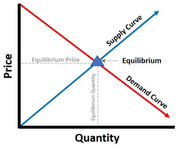
Demand curves will appear somewhat different for each product. They may appear relatively steep or flat, or they may be straight or curved. Nearly all demand curves share the fundamental similarity that they slope down from left to right. Demand curves embody the law of demand: As the price increases, the quantity demanded decreases, and conversely, as the price decreases, the quantity demanded increases. Note that the demand is not the same as quantity demanded – demand refers to the curve and quantity demanded refers to the (specific) point on the curve. Similarly, supply curves will appear somewhat different for each product. They may appear relatively steep or flat, or they may be straight or curved. Nearly all supply curves share the fundamental similarity that they slope up from left to right. Supply curves embody the law of supply: As the price increases, the quantity supplied increases, and conversely, as the price decreases, the quantity supplied decreases. Supply refers to the curve and quantity supplied refers to the (specific) point on the curve (Klingensmith, 2019).
A decrease in demand will shift the demand curve to the left, and lead to a decrease in the equilibrium price and quantity (Stansak, 2024):
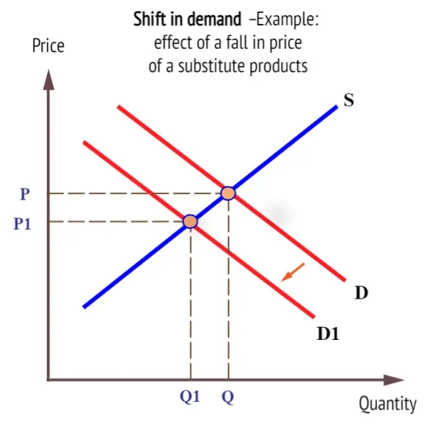
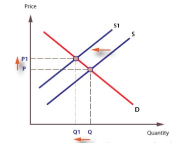
whereas a decrease in supply, will lead to a higher equilibrium price. For instance, if the price of oil increases (or supply decreases), it will lead to a leftward shift in the supply curve, thereby increasing price, but decreasing quantity, resulting in lower demand.
Marginal cost can be shown in the supply-demand graph as follows (Dummies, 2021):
Area under different parts of the supply-demand curves can be used to calculate four measures that can be represented geometrically: equilibrium revenue, consumer surplus, producer surplus and unmet demand as shown in the following figures (MBA Math, n.d.):
Equilibrium revenue here is simply the rectangular area: equilibrium price x equilibrium quantity
Consumer surplus indicates where consumers paid more than the equilibrium price, possibly as a result of successful marketing campaigns. Could have been something like a premium product, a premium sales channel, or the first launch of a new product (think first Tesla buyers).
Counterpart to consumer surplus is producer surplus where some suppliers were willing to supply at a lower price than equilibrium price, at least in some quantity. This leads to different pricing strategies and identify efficiency gains in the marketplace to lower prices for the consumer.
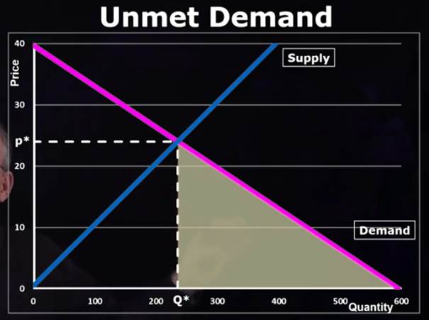
Unmet demand shows where consumers are interested, but unwilling or unable to pay the equilibrium price. These consumers are not in the TR calculation, and presents an area for creative innovation on how to provide something at the lower prices, and perhaps bring these consumers back to main TR marketplace later.
References:
Dummies. (2021, September 27). How to determine marginal cost, marginal revenue, and marginal profit in economics. Retrieved from https://www.dummies.com/article/business-careers-money/business/economics/how-to-determine-marginal-cost-marginal-revenue-and-marginal-profit-in-economics-192262/
Klingensmith, J. Z. (2019, August 26). Chapter 3: Supply and demand. In Introduction to Microeconomics. Affordable Course Transformation: The Pennsylvania State University. Retrieved January 17, 2025, from https://psu.pb.unizin.org/introductiontomicroeconomics/chapter/chapter-3-supply-and-demand/
MBA Math. (n.d.). Supply and demand. Retrieved January 16, 2025, from https://www.mbamath.com
Pingley, A. (2023, May 7). From boring to brilliant: How math makes supply & demand curves fascinating. Medium. Retrieved January 16, 2025, from https://medium.com/techanic/from-boring-to-brilliant-how-math-makes-supply-demand-curves-fascinating-111eab4b91aa
Stansak, J. (2024, June 18). Market disequilibrium and changes in equilibrium. Fiveable. https://library.fiveable.me/ap-micro/unit-2/market-disequilibrium-changes-equilibrium/study-guide/CNeo6STs8jBn29Gawwze

Leave a comment